
Introduction
In physics, expressing natural phenomena in the form of equations and working to solve them is a fundamental intellectual pursuit.
A famous example is Newton’s law of universal gravitation: starting from the observation of an apple falling to the ground, he postulated the force acting on the apple, formulated the corresponding equations, and demonstrated that the motion derived from them also governs celestial bodies like the Moon.
As shown above, if the laws underlying natural phenomena are clarified and expressed as equations, we can predict and explain related phenomena.
Fluid dynamics has evolved along these lines.
However, as the field has become more advanced, a major challenge has emerged: the equations are far too complex to solve by hand.
The Navier-Stokes equations are shown below. Even just looking at their length, you can get a sense of their immense complexity.
\(\frac{D\boldsymbol{v}}{Dt} = -\frac{1}{\rho} \operatorname{grad} p+\frac{\mu}{\rho}\Delta\boldsymbol{v}+\frac{\chi +\frac{1}{3}\, \mu}{\rho} \operatorname{grad} \Theta
+\frac{\Theta}{\rho} \operatorname{grad}(\chi +\frac{1}{3}\, \mu) \)
\(+\frac{1}{\rho} \operatorname{grad}(\boldsymbol{v}\cdot \operatorname{grad} \mu)+\frac{1}{\rho} \operatorname{rot}(\boldsymbol{v}\times \operatorname{grad} \mu)-\frac{1}{\rho}\, \boldsymbol{v} \Delta\mu +\boldsymbol{g} \)
Several approaches have been proposed to address the problem. One such method is Computational Fluid Dynamics (CFD), which has evolved alongside computer technology and is now an indispensable tool in both R&D and design fields.
However, conventionally, the approach was to simplify the equations by removing terms that are irrelevant to the specific flow field being studied.
Therefore, finding ways to analyze flow characteristics easily and efficiently has been of great importance.
What is non-dimensional numbers?
This is where non-dimensional numbers play a key role.
By plugging flow parameters—such as pressure, velocity, viscosity, and thermal conductivity—into non-dimensional numbers, we can determine the fundamental nature of the flow.
While there are numerous non-dimensional numbers, this article focuses on those that are commonly used in the fields of fluid dynamics and heat transfer.
Reynolds Number
The Reynolds Number (Re) is one of the most well-known non-dimensional numbers.
Re represents the ratio of inertial forces, which tend to keep the fluid in motion, to viscous forces, which act to resist that motion. Think of it like the accelerator and the brake of a car.
By calculating the Reynolds Number and comparing the threshold; the critical Reynolds Number, we can determine whether the flow is laminar or turbulent.
\(Re = \dfrac{ρuL}{μ} \)
\(ρ \text{:density}\rm{[kg/m^2]} \)
\(u \text{:velocity}\rm{[m/s]} \)
\(L \text{:characteristic length}\rm{[m]} \)
\(μ \text{:viscosity coefficient}\rm{[kg/(m・s)]} \)
In the case of pipe flow, it is well known that the flow transitions to turbulent if the Reynolds Number exceeds 2300.
Prandtl Number
The Prandtl Number (Pr) is a non-dimensional number named after Ludwig Prandtl, a German physicist and a pioneer of boundary layer theory. This number represents the ratio between the velocity boundary layer and the thermal boundary layer thickness.
\(Pr = \dfrac{ν}{α} = \dfrac{μC_p}{k} \)
\(ν \text{:kinematic viscosity}\rm{[m^2/s]} \)
\(α \text{:thermal diffusivity}\rm{[m^2/s]} \)
\(μ \text{:viscosity coefficient}\rm{[kg/(m・s)]} \)
\(C_p \text{:specific heat at constant pressure}\rm{[J/(kg・K)]} \)
\(k \text{:thermal conductivity}\rm{[J/(m・s・K)]} \)
To add a brief explanation of boundary layers: near a wall surface, the flow slows down due to friction. This slowed-down region forms a layer along the wall, developing at the interface between the main flow and the surface. This is why it is called the “velocity boundary layer”.
Similarly, if there is a temperature difference between the fluid and the wall, a boundary layer also develops for temperature. This is known as the “thermal boundary layer”.
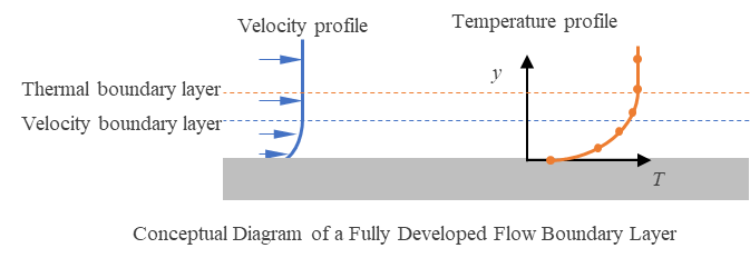
Since the thickness of a boundary layer is determined by the fluid’s inherent physical properties, the Prandtl number is also a fluid-specific value.
(cf. The Reynolds number, by contrast, varies depending on the conditions of the flow field.)
For example, a highly viscous fluid generates stronger friction against the wall surface, resulting in a thicker velocity boundary layer. On the other hand, if a fluid conducts heat easily, the temperature from the wall quickly reaches the main flow, making the thermal boundary layer thinner.
Therefore, under the same flow conditions, a fluid that stays near the wall longer and transfers heat faster—specifically, a fluid with a Prandtl number greater than 1 (Velocity Boundary Layer > Thermal Boundary Layer)—is more advantageous for heat transfer.
Mach Number
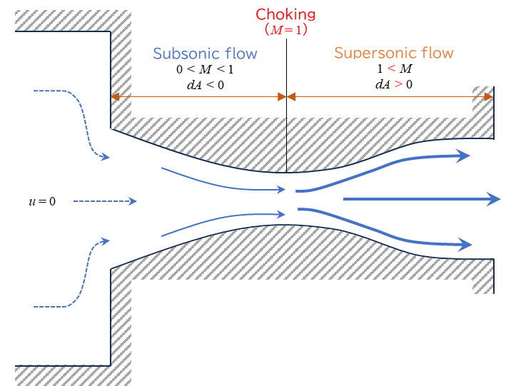
The Mach number represents the ratio of the fluid’s inertial force to its elastic force (the force required to compress the flow).
In other words, a higher Mach number means a stronger driving force behind the flow, indicating that the fluid itself is more easily compressed.
\(Ma = \dfrac{u}{a} \)
\(u \text{:Flow velocity}\rm{[m/s]} \)
\(a \text{:Speed of sound}\rm{[m/s]} \)
When the Mach number is less than 0.3, the fluid undergoes very little compression even if it is blocked or brought to a halt. Therefore, it is perfectly acceptable to calculate the flow assuming a constant density (meaning it can be treated as an incompressible fluid).
However, once it exceeds 0.3, the effects of compressibility can no longer be ignored. When it surpasses 1, the flow enters a state known as supersonic, and various fluid behaviors change drastically.
Nusselt Number
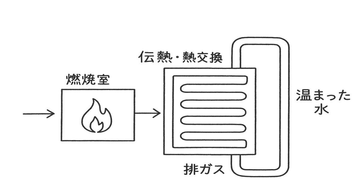
The Nusselt number represents the ratio of convective heat transfer to conductive heat transfer. It also approximately represents the ratio of the characteristic length of an object to the thickness of the thermal boundary layer.
\(Nu = \dfrac{hL}{k} ≅ \dfrac{L}{δ_T} \)
\(h \text{:Heat transfer coefficien}\rm{[J/(m^2・s・K)]} \)
\(L \text{:Characteristic length}\rm{[m]} \)
\(k \text{:Thermal conductivity}\rm{[J/(m・s・K)]} \)
\(δ_T \text{:Thermal boundary layer thickness}\rm{[m]} \)
The Nusselt number is used differently from other non-dimensional numbers; its primary purpose is to determine the heat transfer coefficient.
Specifically, the workflow involves first calculating the Reynolds and Prandtl numbers, estimating the Nusselt number using empirical formulas, and then working backward using the definition above to find the heat transfer coefficient.
For more details, please refer to the article “Heat Transfer Calculation (Double-Pipe Heat Exchanger Design).”
Conclusion
Did you find this article helpful?
We hope it provides a clearer understanding for those who find the non-dimensional numbers challenging.
For more detailed information and derivation methods, please refer to the following references.

コメント